ggplot Basics

library(tidyverse)

Aesthetic Mappings

In ggplot, there are certain aesthetics that can be mapped to the data of a visualization. Some of these aesthetics are:

• Size (in millimeters)
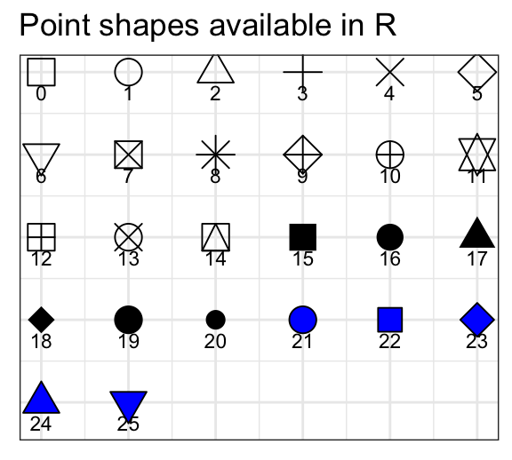
• Shape (from 0 to 25, see below)
• Color
• Fill
• Alpha Transparency (from 0 to 1)

Aesthetics can be mapped uniformly to all data, or split up according to certain categorical observations that exist within the data set.

This applies to all aesthetic values that can be altered.

# Uniform
ggplot(data = mpg, aes(x = hwy,
                       y = displ)) +
  geom_point(color = "blue")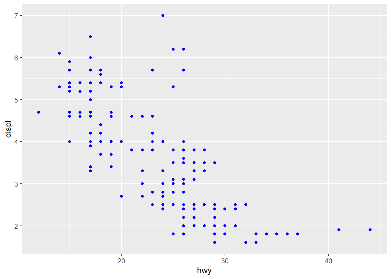

# Split
ggplot(data = mpg, aes(x = hwy,
                       y = displ,
                       color = class)) +
  geom_point()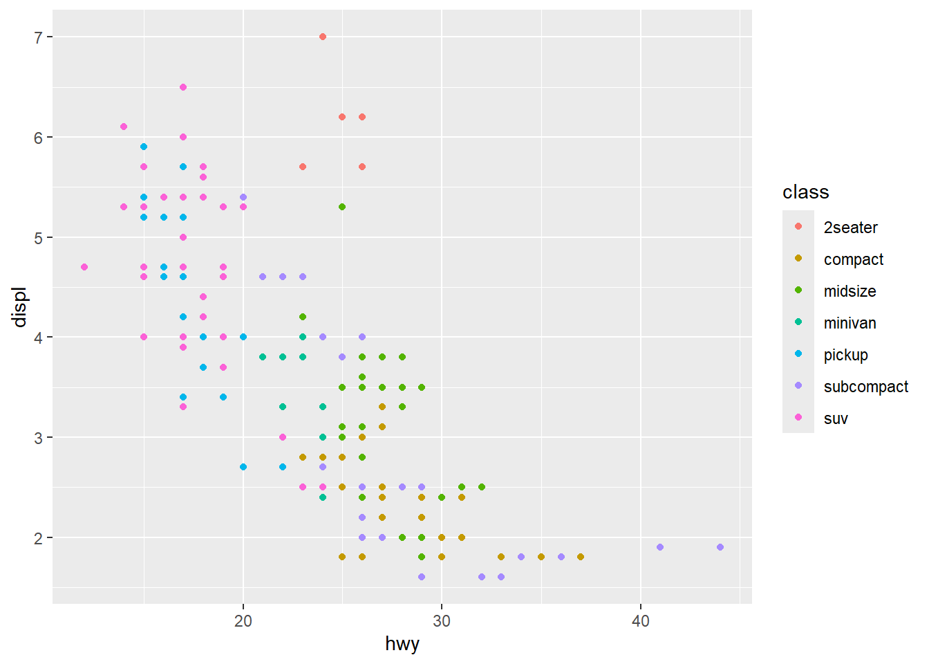

Facet Wrapping

To split our visualization by a certain categorical variable, we can use facet_wrap(~var)

ggplot(data = mpg) + 
  geom_point(mapping = 
               aes(x = displ, 
                   y = hwy), 
             alpha = .5) + 
  facet_wrap(~class)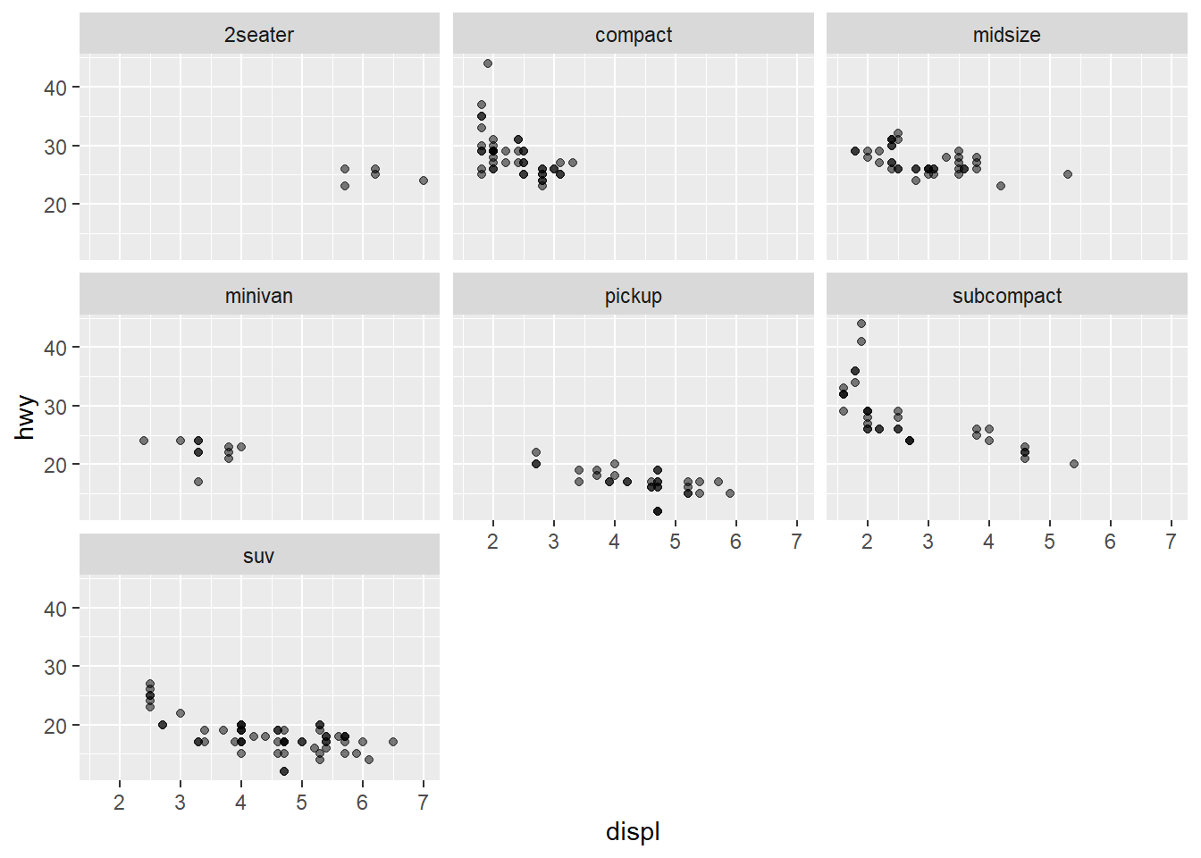

Similarly, we can split a visualization across 2 variables using facet_grid(var1~var2)

ggplot(data = mpg) + 
  geom_point(mapping = 
               aes(x = displ, 
                   y = hwy),
             alpha = .5) + 
  facet_grid(drv ~ cyl)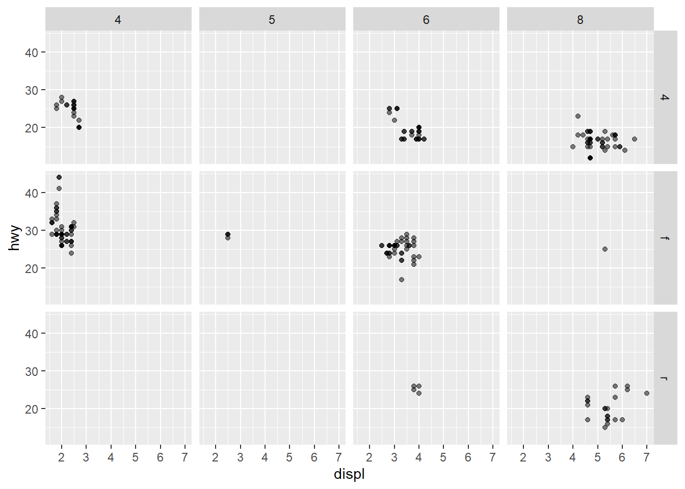

Geometric Objects

Using the different kinds of geom_*() functions, we can visualize data in multiple ways

Examples of geom_*() functions:

• geom_bar(): Bar Chart
• geom_histogram(): Histogram
• geom_line(): Line Graph
• geom_boxplot(): Box Plot
• geom_point(): Scatterplot
• geom_smooth(): Fitted Line (with error range)

Multiple of each geom_*() can be used in a visualization to represent data differently

Statistical Transformations

There are many ways that data can be represented / changed in order to better convey the point you are trying to show through a visualization. We may employ a log transformation on data sets with larger values to better visualize smaller (%) changes, for example.

sale_df <- read_csv("https://bcdanl.github.io/data/home_sales_nyc.csv")

# Without transformation
ggplot(data=sale_df, aes(x=sale_price), bins = 500) +
  geom_histogram()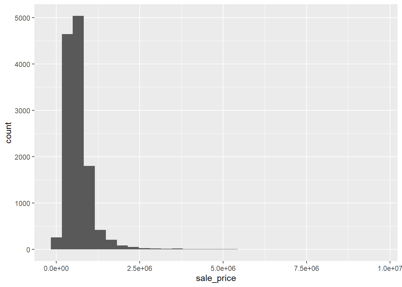

# With transformation
ggplot(data=sale_df, aes(x=log(sale_price)), bins = 500) +
  geom_histogram()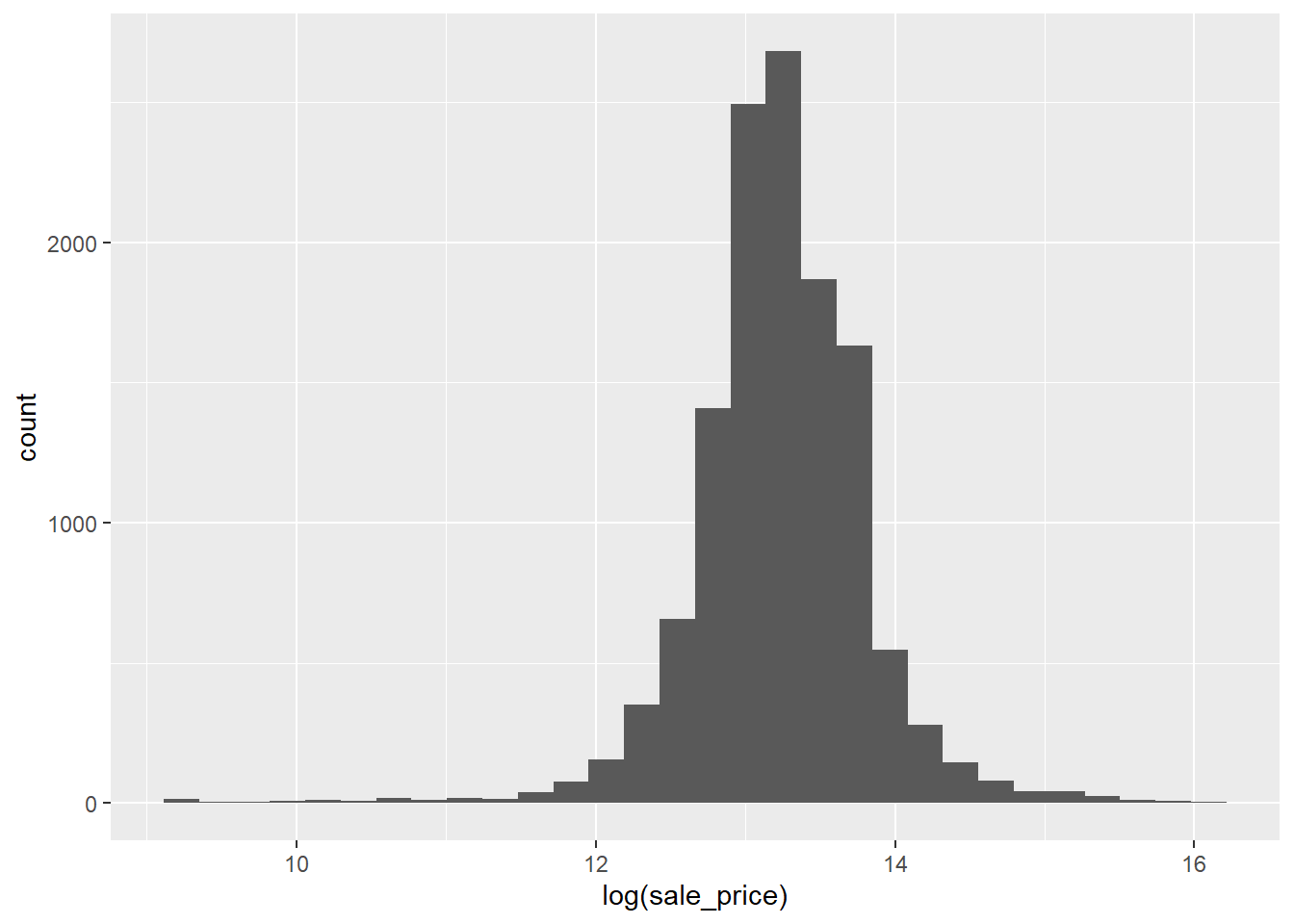

With transformations, large values and skewed data become much more interpretable.

Count vs. Proportion

With geometric objects that count the number of instances for a value (such as geom_bar() or geom_histogram()), we can also use a proportion of the entire data set to represent the data with after_stat() or stat()

ggplot(data = diamonds) + 
  geom_bar(mapping = 
             aes(x = cut))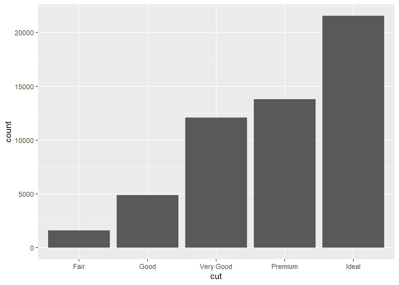

ggplot(data = diamonds) + 
  geom_bar(mapping = 
             aes(x = cut, 
                 y = after_stat(prop), 
                 group = 1))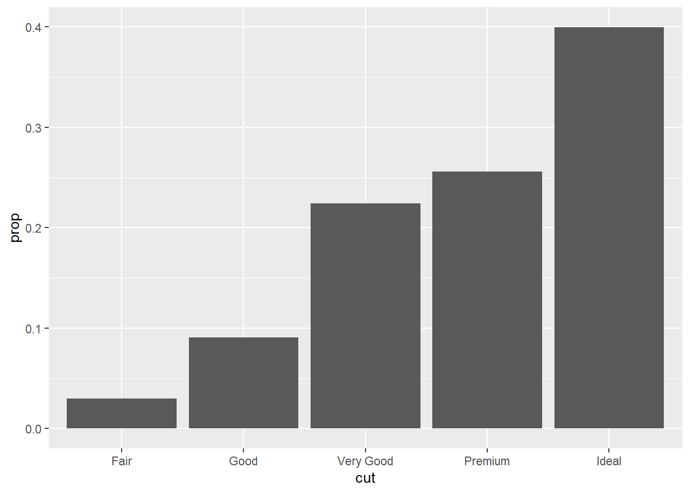

Position Adjustment

Some geometric objects have the ability to have their ‘positions’ adjusted, meaning that they are able to be further split categorically in multiple ways.

# No Adjustment
ggplot(data = diamonds) + 
  geom_bar(mapping = 
             aes(x = cut, 
                 fill = cut))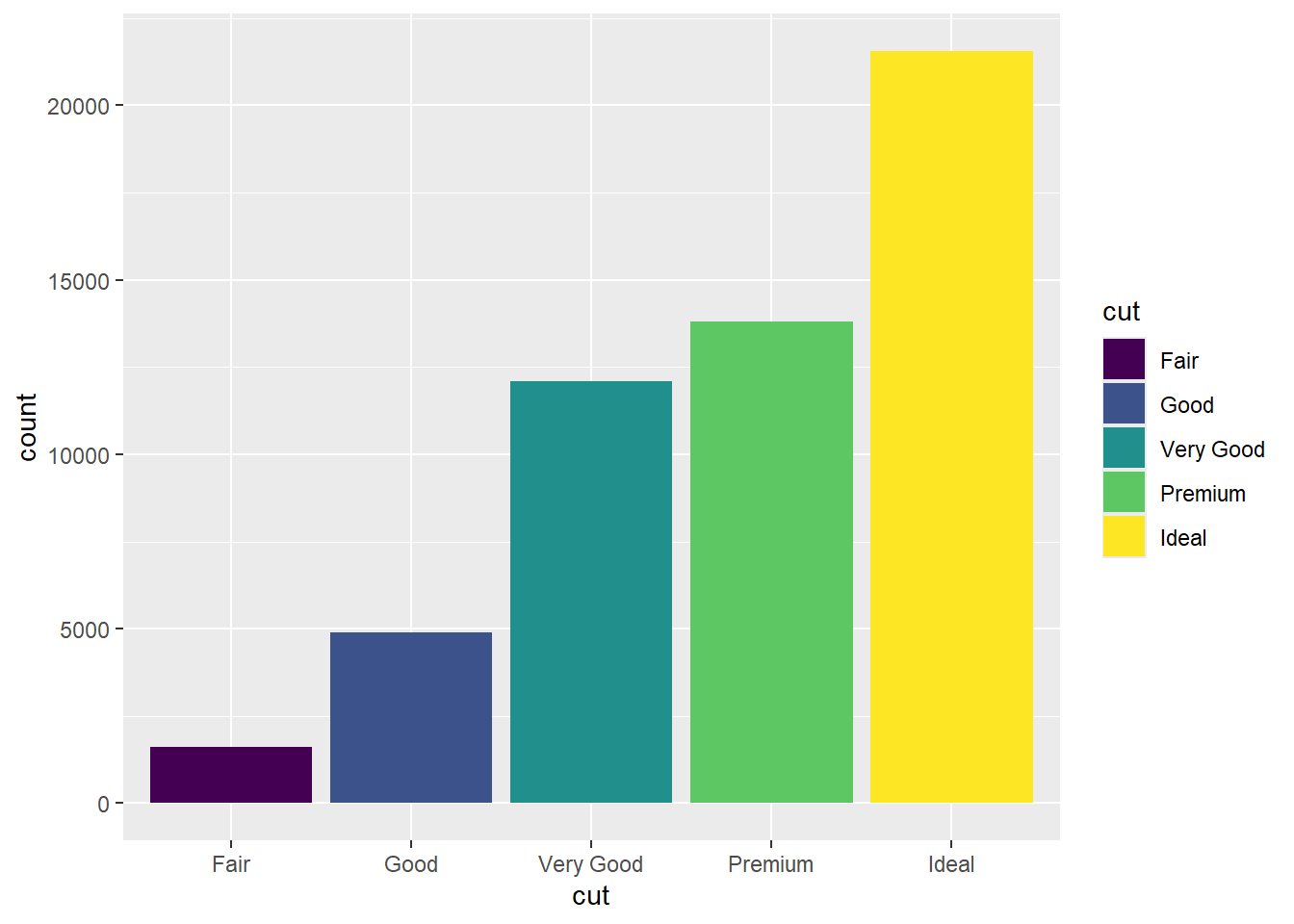

# Position = 'stack'
ggplot(data = diamonds) + 
  geom_bar(mapping = 
             aes(x = cut, 
                 fill = clarity),
           position = "stack")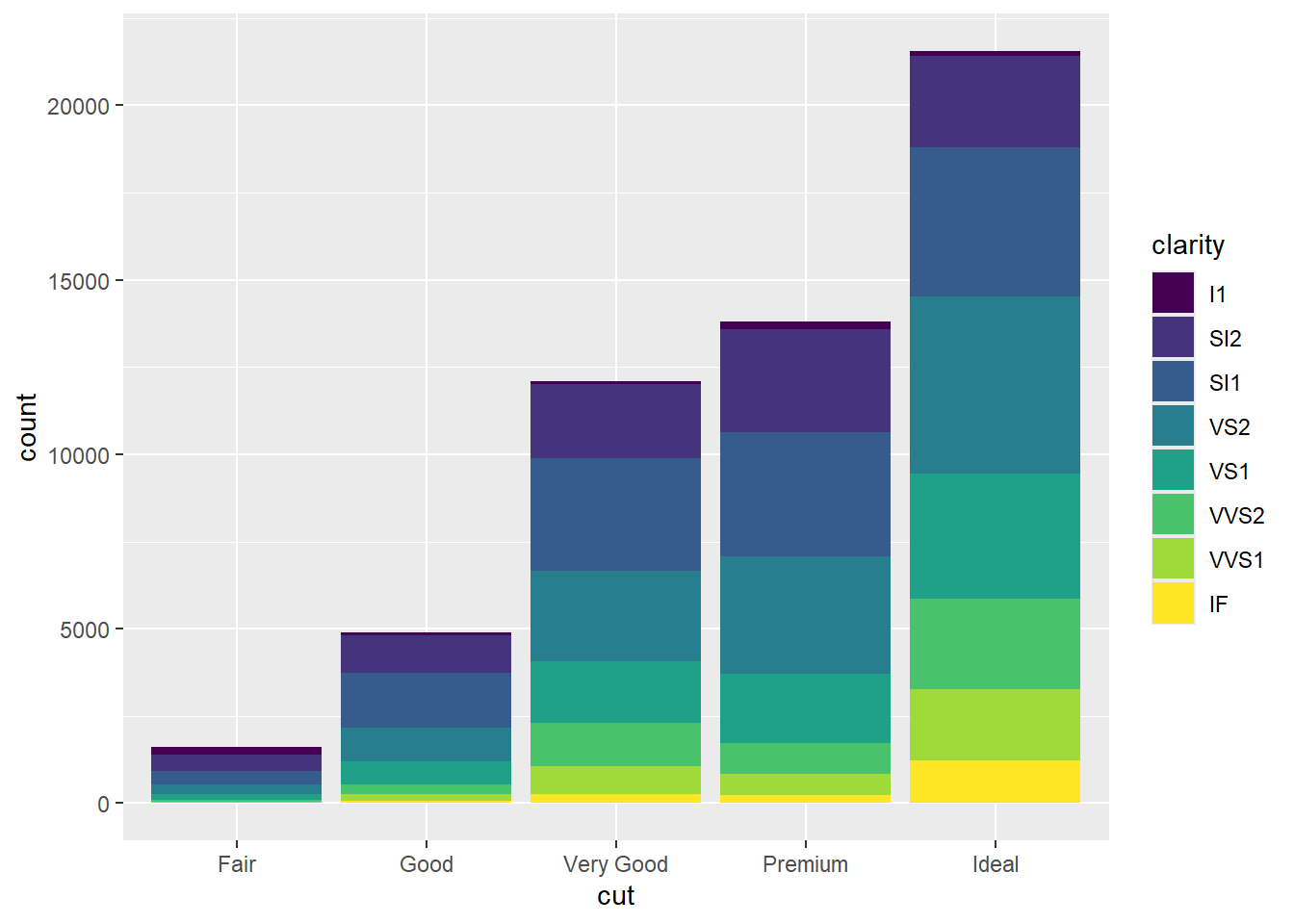

# Position = "dodge"
ggplot(data = diamonds) + 
  geom_bar(mapping = 
             aes(x = cut, 
                 fill = clarity),
           position = "dodge")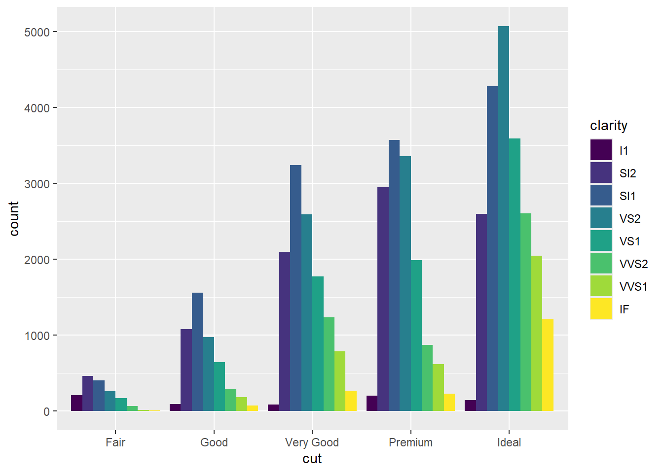

# Position = 'fill'
ggplot(data = diamonds) + 
  geom_bar(mapping = 
             aes(x = cut, 
                 fill = clarity),
           position = "fill")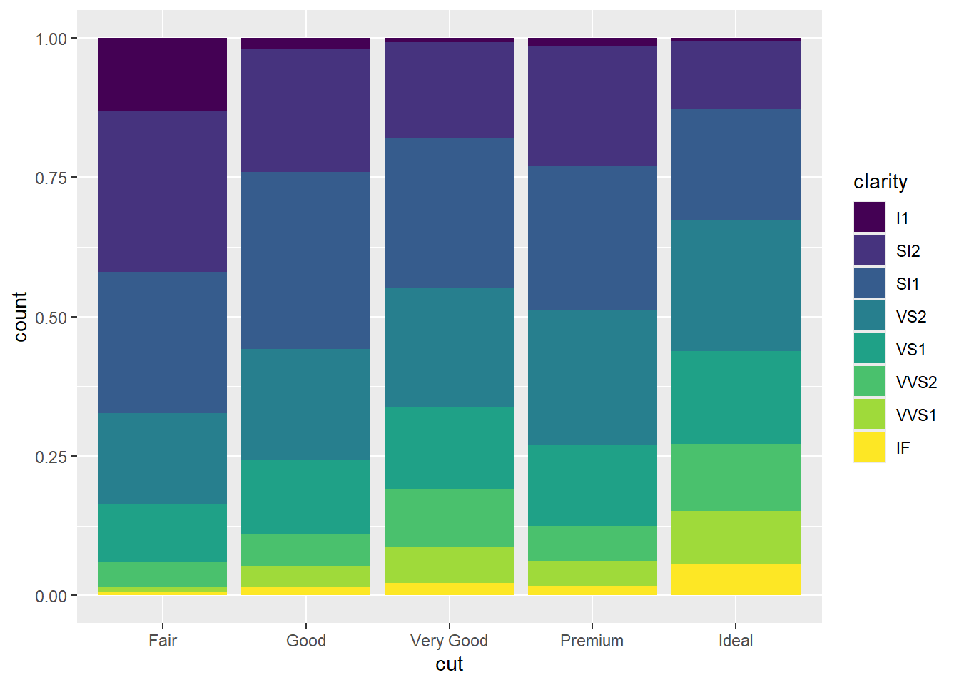

ggplot Grammar

• DATA
• GEOM_FUNCTION
• MAPPINGS
• STAT
• POSITION
• COORDINATE_FUNCTION
• FACET_FUNCTION
• SCALE_FUNCTIONS
• GUIDES
• THEME

ggplot Themes

To assist in presentation and accessibility, there are themes that alter the coloration of a visualization. For example:

• theme_gray()
• theme_bw()
• theme_linedraw()
• theme_light()
• theme_dark()
• theme_minimal()
• theme_classic()
• theme_void()
• theme_test()

The ggthemes package comes with some additional themes:

• theme_economist()
• theme_wsj()
• theme_fivethirtyeight()
• theme_map()

There are also color palettes that allow for increased accessibility for the colorblind, such as:

• scale_color_tableau()
• scale_color_colorblind()

Saving plots

We can use ggsave() to save a ggplot output as a .png or .pdf file

• Syntax: ggsave(filename = “—.png”, plot = —)

Optionally, we can alter the dimensions of the figure being output

• ggsave(‘filename.png’, plot = —, height = —, width = —, units = —)